Exploratory analysis of London street level crime 2015-2017
- 16 mins
import pandas as pd
import numpy as np
import matplotlib.pyplot as plt
plt.style.use('ggplot')
%matplotlib inline
Lets load the dataset
data source : https://data.police.uk/data/archive/
data = pd.read_csv('crime.csv')
check the number of rows in the dataset
data.shape
(18000, 13)
the dataset has 18,000 rows and 13 columns
lets check the first five rows
data.iloc[:5,:]
| Unnamed: 0 | Crime ID | Month | Reported by | Falls within | Longitude | Latitude | Location | LSOA code | LSOA name | Crime type | Last outcome category | Context | |
|---|---|---|---|---|---|---|---|---|---|---|---|---|---|
| 0 | 0 | 80e07583f4bd74b85e457d92eef5d014e4e8d7b0eab0dc... | 2015-01 | City of London Police | City of London Police | -0.106453 | 51.518207 | On or near Charterhouse Street | E01000916 | Camden 027B | Bicycle theft | Unable to prosecute suspect | NaN |
| 1 | 1 | 6589894ebc515f501527628eb650d52a6f031116eb0ada... | 2015-01 | City of London Police | City of London Police | -0.111497 | 51.518226 | On or near Pedestrian Subway | E01000914 | Camden 028B | Burglary | Investigation complete; no suspect identified | NaN |
| 2 | 2 | e6dc6a4a33ed886c7c72beaff0c5de92cc35cd2f76c6e5... | 2015-01 | City of London Police | City of London Police | -0.111497 | 51.518226 | On or near Pedestrian Subway | E01000914 | Camden 028B | Burglary | Unable to prosecute suspect | NaN |
| 3 | 3 | b6e6462d45d0d7f4258d57628cab4c8988dc41ac675b63... | 2015-01 | City of London Police | City of London Police | -0.111497 | 51.518226 | On or near Pedestrian Subway | E01000914 | Camden 028B | Other theft | Investigation complete; no suspect identified | NaN |
| 4 | 4 | 769e1aa86e62b5f3c4c08c8c140147a275ca721d0801ba... | 2015-01 | City of London Police | City of London Police | -0.113767 | 51.517372 | On or near Stone Buildings | E01000914 | Camden 028B | Theft from the person | Investigation complete; no suspect identified | NaN |
lets remove the crime Id and unamed 0 columns
del data['Crime ID']
del data['Unnamed: 0']
data.head(3)
| Month | Reported by | Falls within | Longitude | Latitude | Location | LSOA code | LSOA name | Crime type | Last outcome category | Context | |
|---|---|---|---|---|---|---|---|---|---|---|---|
| 0 | 2015-01 | City of London Police | City of London Police | -0.106453 | 51.518207 | On or near Charterhouse Street | E01000916 | Camden 027B | Bicycle theft | Unable to prosecute suspect | NaN |
| 1 | 2015-01 | City of London Police | City of London Police | -0.111497 | 51.518226 | On or near Pedestrian Subway | E01000914 | Camden 028B | Burglary | Investigation complete; no suspect identified | NaN |
| 2 | 2015-01 | City of London Police | City of London Police | -0.111497 | 51.518226 | On or near Pedestrian Subway | E01000914 | Camden 028B | Burglary | Unable to prosecute suspect | NaN |
lets check the month datatype
data.info()
<class 'pandas.core.frame.DataFrame'>
RangeIndex: 18000 entries, 0 to 17999
Data columns (total 11 columns):
Month                    18000 non-null object
Reported by              18000 non-null object
Falls within             18000 non-null object
Longitude                17129 non-null float64
Latitude                 17129 non-null float64
Location                 18000 non-null object
LSOA code                17129 non-null object
LSOA name                17129 non-null object
Crime type               18000 non-null object
Last outcome category    14801 non-null object
Context                  0 non-null float64
dtypes: float64(3), object(8)
memory usage: 984.4+ KB
it appears the month datatype is object, we need to convert it to datetime to be able to manipulate it
import datetime
data['Month'] = pd.to_datetime(data['Month'],yearfirst=True)
data.info()
<class 'pandas.core.frame.DataFrame'>
RangeIndex: 18000 entries, 0 to 17999
Data columns (total 11 columns):
Month                    18000 non-null datetime64[ns]
Reported by              18000 non-null object
Falls within             18000 non-null object
Longitude                17129 non-null float64
Latitude                 17129 non-null float64
Location                 18000 non-null object
LSOA code                17129 non-null object
LSOA name                17129 non-null object
Crime type               18000 non-null object
Last outcome category    14801 non-null object
Context                  0 non-null float64
dtypes: datetime64[ns](1), float64(3), object(7)
memory usage: 1.0+ MB
lest check location based on incicence of crime
data.Location.value_counts()
No Location                                871
On or near Police Station                  607
On or near Pedestrian Subway               607
On or near Supermarket                     532
On or near Parking Area                    487
On or near Great St Helen'S                354
On or near Conference/Exhibition Centre    318
On or near Nightclub                       316
On or near Blomfield Street                304
On or near Queen Victoria Street           297
On or near St Martin'S Le Grand            296
On or near Bride Lane                      296
On or near New Change                      284
On or near Shopping Area                   274
On or near Fish Street Hill                269
On or near Clement'S Lane                  235
On or near Gracechurch Street              204
On or near Fleet Street                    194
On or near Artillery Lane                  172
On or near Leadenhall Street               166
On or near Fetter Lane                     158
On or near Finch Lane                      149
On or near Philpot Lane                    149
On or near Bow Lane                        141
On or near Cheapside                       139
On or near Bell Inn Yard                   138
On or near Bishopsgate                     133
On or near Bear Alley                      132
On or near Primrose Street                 130
On or near Eastcheap                       129
                                          ...
On or near St Dunstan'S Lane                 3
On or near Mount Pleasant                    3
On or near Old Buildings                     2
On or near Dysart Street                     2
On or near Amen Court                        2
On or near Sandy Lane                        2
On or near Tooley Street                     2
On or near Shadwell Gardens                  2
On or near Goswell Place                     2
On or near Mark Street                       1
On or near Milk Street                       1
On or near Little Essex Street               1
On or near Farringdon Street                 1
On or near Cripplegate Street                1
On or near Timber Street                     1
On or near Goldsmith Street                  1
On or near Stoney Lane                       1
On or near Fournier Street                   1
On or near Nelson Terrace                    1
On or near Whiskin Street                    1
On or near Queen Street Place                1
On or near Tower Royal                       1
On or near Mucking Wharf Road                1
On or near Folgate Street                    1
On or near Holywell Row                      1
On or near Banner Street                     1
On or near Upper Ground                      1
On or near Haven Quays                       1
On or near Weaver'S Lane                     1
On or near Bartlett Court                    1
Name: Location, Length: 335, dtype: int64
lets visualize top ten crime location
def adjust_plot(ax):
    plt.rc('xtick',labelsize=22)
    plt.rc('ytick',labelsize=22)
# create a list to collect the plt.patches data
totals = []

# find the values and append to list
for i in ax.patches:
    totals.append(i.get_height())

# set individual bar lables using above list
total = sum(totals)

# set individual bar lables using above list
for i in ax.patches:
    # get_x pulls left or right; get_height pushes up or down
    ax.text(i.get_x()-.03, i.get_height()+.5, \
            str(round((i.get_height()/total)*100, 2))+'%', fontsize=15,
                color='black')
ax = data.Location.value_counts().head(10).plot(kind='bar',figsize=(15,6),title='Crime Location in London city')
plt.title("Crime Location in London 2015-2017", fontname='Ubuntu', fontsize=18,
            fontstyle='italic', fontweight='bold',color='green')
adjust_plot()
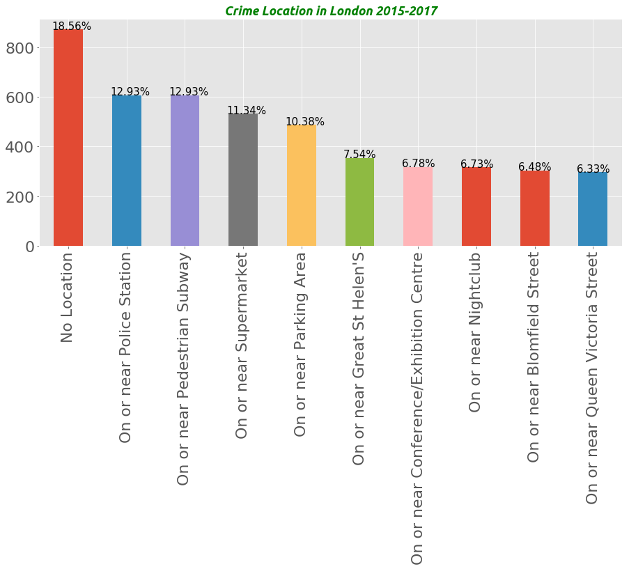
it turned out location was unknown for 871 times.Aside from No location, most crime happnede very close to police station!!!
lets visualize the 5 least crime location
data.Location.value_counts().tail(5).plot(kind='bar',figsize=(13,5))
<matplotlib.axes._subplots.AxesSubplot at 0xacba93ec>
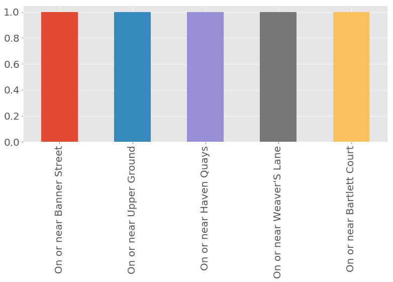
we found that the most crime free location are Banner Street,Upper Ground,Weaver’s Lane
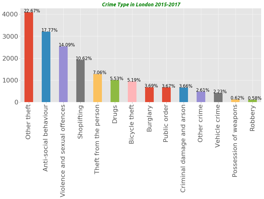
lets check crime type
data['Crime type'].value_counts()
Other theft                     4081
Anti-social behaviour           3199
Violence and sexual offences    2536
Shoplifting                     1911
Theft from the person           1270
Drugs                            996
Bicycle theft                    934
Burglary                         665
Public order                     661
Criminal damage and arson        659
Other crime                      470
Vehicle crime                    402
Possession of weapons            111
Robbery                          105
Name: Crime type, dtype: int64
other theft, Anti Social behaviour and Sexual behavoiurs is the most prevalent
ax = data['Crime type'].value_counts().plot(kind='bar',figsize=(15,6),title='Crime type in Londo--2015-2017')
plt.title("Crime Type in London 2015-2017", fontname='Ubuntu', fontsize=18,
            fontstyle='italic', fontweight='bold',color='green')
adjust_plot(ax)
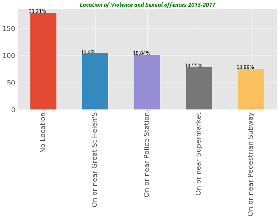
Location in which Violence and Sexual offences occur the most
data[data['Crime type'] == 'Violence and sexual offences']['Location'].value_counts()
No Location                                178
On or near Great St Helen'S                104
On or near Police Station                  101
On or near Supermarket                      78
On or near Pedestrian Subway                75
On or near Nightclub                        65
On or near Parking Area                     64
On or near Conference/Exhibition Centre     55
On or near Blomfield Street                 53
On or near Queen Victoria Street            51
On or near Leadenhall Street                50
On or near Fish Street Hill                 43
On or near Shopping Area                    34
On or near Philpot Lane                     33
On or near Moorgate                         32
On or near Wormwood Street                  30
On or near Gracechurch Street               30
On or near St Martin'S Le Grand             29
On or near Finch Lane                       29
On or near Bride Lane                       29
On or near Watling Court                    28
On or near St Swithin'S Lane                27
On or near New Broad Street                 25
On or near New Change                       23
On or near Wood Street                      23
On or near Mark Lane                        21
On or near Moor Lane                        20
On or near Camomile Street                  20
On or near Distaff Lane                     20
On or near Creed Lane                       19
                                          ...
On or near Arthur Street                     1
On or near Fournier Street                   1
On or near Cloth Street                      1
On or near Old Seacoal Lane                  1
On or near Lloyd'S Avenue                    1
On or near Bell Yard                         1
On or near Sandy'S Row                       1
On or near Cursitor Street                   1
On or near Amen Corner                       1
On or near Norton Folgate                    1
On or near St Dunstan'S Hill                 1
On or near St Mary Axe                       1
On or near Copthall Avenue                   1
On or near Leadenhall Place                  1
On or near Monkwell Square                   1
On or near Tudor Street                      1
On or near Lombard Lane                      1
On or near Portsoken Street                  1
On or near Pilgrim Street                    1
On or near Nun Court                         1
On or near Temple Lane                       1
On or near South Place Mews                  1
On or near John Carpenter Street             1
On or near Basinghall Street                 1
On or near King'S Arms Yard                  1
On or near Charterhouse Street               1
On or near Moorgate Place                    1
On or near Old Square                        1
On or near Billiter Street                   1
On or near Charterhouse Mews                 1
Name: Location, Length: 256, dtype: int64
sex_crime = data[data['Crime type'] == 'Violence and sexual offences']['Location'].value_counts()
ax = sex_crime.head().plot(kind='bar',figsize=(15,6),title='Location of Violence and Sexual Offence')
plt.title("Location of Violence and Sexual offences 2015-2017", fontname='Ubuntu', fontsize=18,
            fontstyle='italic', fontweight='bold',color='green')
adjust_plot(ax)
analysis of crime based on Last outcome category
data['Last outcome category'].value_counts()
Investigation complete; no suspect identified          7568
Unable to prosecute suspect                            1644
Status update unavailable                              1613
Court result unavailable                                783
Offender given a caution                                591
Under investigation                                     531
Offender sent to prison                                 443
Offender given a drugs possession warning               249
Local resolution                                        245
Offender fined                                          198
Offender given suspended prison sentence                143
Offender given community sentence                       138
Formal action is not in the public interest             129
Defendant found not guilty                              116
Awaiting court outcome                                  104
Offender given penalty notice                            85
Offender given conditional discharge                     81
Court case unable to proceed                             42
Offender otherwise dealt with                            27
Suspect charged as part of another case                  22
Further investigation is not in the public interest      21
Offender deprived of property                            12
Action to be taken by another organisation                7
Offender ordered to pay compensation                      5
Defendant sent to Crown Court                             3
Offender given absolute discharge                         1
Name: Last outcome category, dtype: int64
ax = data['Last outcome category'].value_counts().head(10).plot(kind='bar',figsize=(16,7),title='Crime Outome')
adjust_plot(ax)
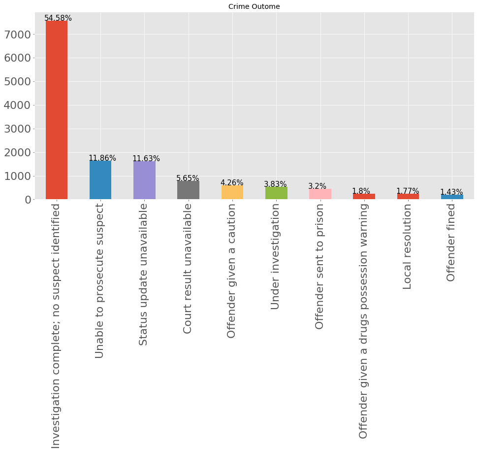
turned out that most time suspect was unable to be indentified
Time series analysis of the crime
crime_time = data['Month']
crime_time.head()
0   2015-01-01
1   2015-01-01
2   2015-01-01
3   2015-01-01
4   2015-01-01
Name: Month, dtype: datetime64[ns]
crime_time = pd.DataFrame(crime_time)
#pd.to_datetime(crime_time['Month'],yearfirst=True)
#crime_time['Month'] = pd.to_datetime(crime_time['Month'],yearfirst=True)
crime_time.head()
| Month | |
|---|---|
| 0 | 2015-01-01 |
| 1 | 2015-01-01 |
| 2 | 2015-01-01 |
| 3 | 2015-01-01 |
| 4 | 2015-01-01 |
crime_time['value'] = 0
crime_time['Month'] = pd.to_datetime(crime_time['Month'],yearfirst=True)
crime_time.set_index(crime_time.Month,inplace=True)
del crime_time['Month']
crime_time.head()
| value | |
|---|---|
| Month | |
| 2015-01-01 | 0 |
| 2015-01-01 | 0 |
| 2015-01-01 | 0 |
| 2015-01-01 | 0 |
| 2015-01-01 | 0 |
crime_t = crime_time.resample('M')
crime_t
DatetimeIndexResampler [freq=<MonthEnd>, axis=0, closed=right, label=right, convention=start, base=0]
#
crime_per_month = crime_t.count()
ax = crime_per_month.plot(kind='line',figsize=(16,7),title='Monthly Times seties (2015-2017)')
adjust_pot(ax)
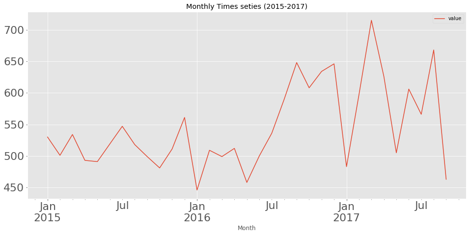
the above show crime was high around march of 2017
crime_w = crime_time.resample('Y')
crime_w = crime_w.count()
crime_w.index.name = 'Year'
crime_w.head()
| value | |
|---|---|
| Year | |
| 2015-12-31 | 6185 |
| 2016-12-31 | 6586 |
| 2017-12-31 | 5229 |
ax = crime_w.plot(figsize=(17,6),title='Yearly Time series of crime per year')
adjust_plot(ax)
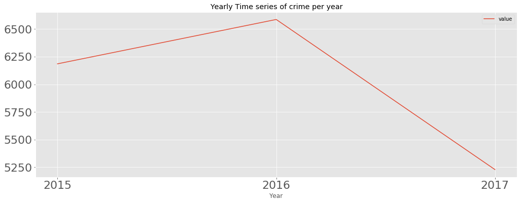
there was more crime in 2016 than 2015 and 2017 but there was a particular month in 2017 that recorded highest crime which was around march
we also learnt that through out 2015 crime rate was on the increase

Mustapha Omotosho
constant learner,machine learning enthusiast,huge Barcelona fan