Restricted Boltzmann Machine for Diabetes Prediction
- 12 minsRestricted Boltzmann machine (RBM)
A restricted Boltzmann machine (RBM) is a generative stochastic artificial neural network that can learn a probability distribution over its set of inputs.It has seen wide applications in different areas of supervised/unsupervised machine learning such as feature learning, dimensionality reduction, classification, collaborative filtering, and topic modeling. Source
Bernoulli RBM
we will use Berrnoulli RBM in scikit learn with Logistic regression.The BernoulliRBM is an unsupervised method so it is mostly used for non-linear feature extraction that can be feed to a classifier (in this case Logistic Regression).
Objective
To train a calssifier for predicting Diabetes
Data source
diabetes data set is included in scikit learn and can also be downloded from the kaggle
The Notebook
The notebook for this work can be found at [Restricted Boltzmann machine (RBM)]
import pandas as pd
import seaborn as sns
import random
from sklearn.model_selection import train_test_split
%matplotlib inline
import matplotlib
import matplotlib.pyplot as plt
from sklearn.preprocessing import MinMaxScaler
from sklearn.preprocessing import StandardScaler
from numpy import set_printoptions
from sklearn.model_selection import KFold
from sklearn.model_selection import cross_val_score
from sklearn.pipeline import Pipeline
from sklearn.neural_network import BernoulliRBM
from sklearn import metrics
from sklearn.linear_model import LogisticRegression
from sklearn.grid_search import GridSearchCV
import matplotlib.pyplot as plt
from sklearn.metrics import confusion_matrix
from sklearn.metrics import classification_report
from sklearn.metrics import classification_report
data = pd.read_csv('Diabetes.csv')
Dimensions of Your Data
shape = data.shape
print(shape)
(768, 9)
data.head()
| preg_count | glucose_concentration | blood_pressure | skin_thickness | serum_insulin | bmi | pedigree_function | age | class | |
|---|---|---|---|---|---|---|---|---|---|
| 0 | 6 | 148 | 72 | 35 | 0 | 33.6 | 0.627 | 50 | 1 |
| 1 | 1 | 85 | 66 | 29 | 0 | 26.6 | 0.351 | 31 | 0 |
| 2 | 8 | 183 | 64 | 0 | 0 | 23.3 | 0.672 | 32 | 1 |
| 3 | 1 | 89 | 66 | 23 | 94 | 28.1 | 0.167 | 21 | 0 |
| 4 | 0 | 137 | 40 | 35 | 168 | 43.1 | 2.288 | 33 | 1 |
Descriptive Statistics
# Statistical Summary
from pandas import set_option
set_option('display.width', 100)
set_option('precision', 3)
description = data.describe()
(description)
| preg_count | glucose_concentration | blood_pressure | skin_thickness | serum_insulin | bmi | pedigree_function | age | class | |
|---|---|---|---|---|---|---|---|---|---|
| count | 768.000 | 768.000 | 768.000 | 768.000 | 768.000 | 768.000 | 768.000 | 768.000 | 768.000 |
| mean | 3.845 | 120.895 | 69.105 | 20.536 | 79.799 | 31.993 | 0.472 | 33.241 | 0.349 |
| std | 3.370 | 31.973 | 19.356 | 15.952 | 115.244 | 7.884 | 0.331 | 11.760 | 0.477 |
| min | 0.000 | 0.000 | 0.000 | 0.000 | 0.000 | 0.000 | 0.078 | 21.000 | 0.000 |
| 25% | 1.000 | 99.000 | 62.000 | 0.000 | 0.000 | 27.300 | 0.244 | 24.000 | 0.000 |
| 50% | 3.000 | 117.000 | 72.000 | 23.000 | 30.500 | 32.000 | 0.372 | 29.000 | 0.000 |
| 75% | 6.000 | 140.250 | 80.000 | 32.000 | 127.250 | 36.600 | 0.626 | 41.000 | 1.000 |
| max | 17.000 | 199.000 | 122.000 | 99.000 | 846.000 | 67.100 | 2.420 | 81.000 | 1.000 |
check if data is balanced
class_counts = data.groupby('class').size()
print(class_counts)
class
0    500
1    268
dtype: int64
Correlations Between Attributes
correlations = data.corr(method='pearson')
(correlations)
| preg_count | glucose_concentration | blood_pressure | skin_thickness | serum_insulin | bmi | pedigree_function | age | class | |
|---|---|---|---|---|---|---|---|---|---|
| preg_count | 1.000 | 0.129 | 0.141 | -0.082 | -0.074 | 0.018 | -0.034 | 0.544 | 0.222 |
| glucose_concentration | 0.129 | 1.000 | 0.153 | 0.057 | 0.331 | 0.221 | 0.137 | 0.264 | 0.467 |
| blood_pressure | 0.141 | 0.153 | 1.000 | 0.207 | 0.089 | 0.282 | 0.041 | 0.240 | 0.065 |
| skin_thickness | -0.082 | 0.057 | 0.207 | 1.000 | 0.437 | 0.393 | 0.184 | -0.114 | 0.075 |
| serum_insulin | -0.074 | 0.331 | 0.089 | 0.437 | 1.000 | 0.198 | 0.185 | -0.042 | 0.131 |
| bmi | 0.018 | 0.221 | 0.282 | 0.393 | 0.198 | 1.000 | 0.141 | 0.036 | 0.293 |
| pedigree_function | -0.034 | 0.137 | 0.041 | 0.184 | 0.185 | 0.141 | 1.000 | 0.034 | 0.174 |
| age | 0.544 | 0.264 | 0.240 | -0.114 | -0.042 | 0.036 | 0.034 | 1.000 | 0.238 |
| class | 0.222 | 0.467 | 0.065 | 0.075 | 0.131 | 0.293 | 0.174 | 0.238 | 1.000 |
skew and Kurtosis of univeraite data
print(data.skew())
preg_count               0.902
glucose_concentration    0.174
blood_pressure          -1.844
skin_thickness           0.109
serum_insulin            2.272
bmi                     -0.429
pedigree_function        1.920
age                      1.130
class                    0.635
dtype: float64
data.kurtosis()
preg_count               0.159
glucose_concentration    0.641
blood_pressure           5.180
skin_thickness          -0.520
serum_insulin            7.214
bmi                      3.290
pedigree_function        5.595
age                      0.643
class                   -1.601
dtype: float64
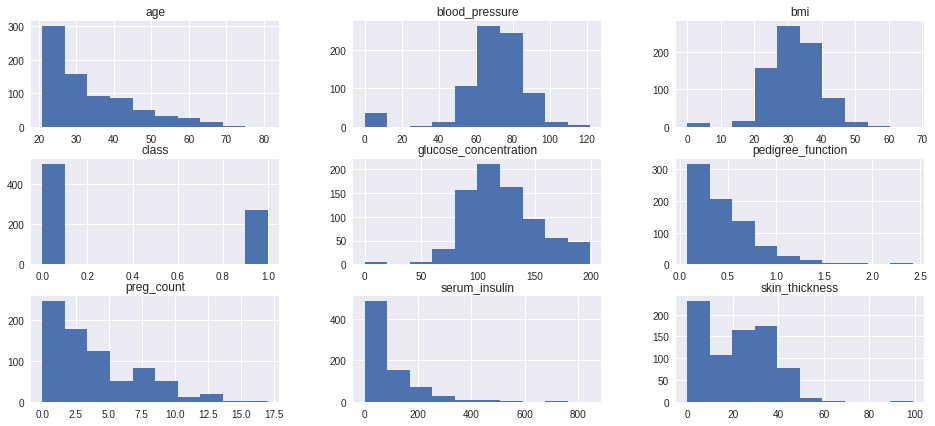
Univariate Visualization
data.hist(figsize=(16,7))
array([[<matplotlib.axes._subplots.AxesSubplot object at 0x7fcb1f381750>,
        <matplotlib.axes._subplots.AxesSubplot object at 0x7fcb1f2de9d0>,
        <matplotlib.axes._subplots.AxesSubplot object at 0x7fcb1f306250>],
       [<matplotlib.axes._subplots.AxesSubplot object at 0x7fcb1ea21dd0>,
        <matplotlib.axes._subplots.AxesSubplot object at 0x7fcb1f2d5b50>,
        <matplotlib.axes._subplots.AxesSubplot object at 0x7fcb1e94ee50>],
       [<matplotlib.axes._subplots.AxesSubplot object at 0x7fcb1e91e290>,
        <matplotlib.axes._subplots.AxesSubplot object at 0x7fcb1e8df990>,
        <matplotlib.axes._subplots.AxesSubplot object at 0x7fcb1e89ef90>]],
      dtype=object)
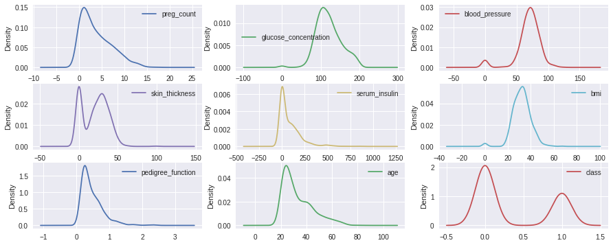
Density Curve to inspect shape of each distribution clearly
data.plot(kind='density', subplots=True, layout=(3,3), sharex=False,figsize=(15,6))
array([[<matplotlib.axes._subplots.AxesSubplot object at 0x7fcb1e69d390>,
        <matplotlib.axes._subplots.AxesSubplot object at 0x7fcb1e63f790>,
        <matplotlib.axes._subplots.AxesSubplot object at 0x7fcb1e600410>],
       [<matplotlib.axes._subplots.AxesSubplot object at 0x7fcb1e5a7350>,
        <matplotlib.axes._subplots.AxesSubplot object at 0x7fcb1e5889d0>,
        <matplotlib.axes._subplots.AxesSubplot object at 0x7fcb1e543a90>],
       [<matplotlib.axes._subplots.AxesSubplot object at 0x7fcb1e48d6d0>,
        <matplotlib.axes._subplots.AxesSubplot object at 0x7fcb1e45c190>,
        <matplotlib.axes._subplots.AxesSubplot object at 0x7fcb1e419d10>]],
      dtype=object)
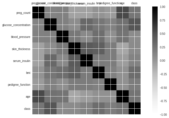
Multivariate Plots
import numpy
correlations = data.corr()
# plot correlation matrix
fig = plt.figure(figsize=(15,7))
ax = fig.add_subplot(111)
cax = ax.matshow(correlations, vmin=-1, vmax=1)
fig.colorbar(cax)
ticks = numpy.arange(0,9,1)
ax.set_xticks(ticks)
ax.set_yticks(ticks)
ax.set_xticklabels(data.columns)
ax.set_yticklabels(data.columns)
plt.show()
Data standardization
# Standardize data (0 mean, 1 stdev)
data_array = data.values
# separate array into input and output components
X = data_array[:,0:8]
Y = data_array[:,8]
scaler = StandardScaler()
scaledX = scaler.fit_transform(X)
# summarize transformed data
set_printoptions(precision=3)
print(scaledX[0:8,:])
[[ 0.64   0.848  0.15   0.907 -0.693  0.204  0.468  1.426]
 [-0.845 -1.123 -0.161  0.531 -0.693 -0.684 -0.365 -0.191]
 [ 1.234  1.944 -0.264 -1.288 -0.693 -1.103  0.604 -0.106]
 [-0.845 -0.998 -0.161  0.155  0.123 -0.494 -0.921 -1.042]
 [-1.142  0.504 -1.505  0.907  0.766  1.41   5.485 -0.02 ]
 [ 0.343 -0.153  0.253 -1.288 -0.693 -0.811 -0.818 -0.276]
 [-0.251 -1.342 -0.988  0.719  0.071 -0.126 -0.676 -0.616]
 [ 1.828 -0.184 -3.573 -1.288 -0.693  0.42  -1.02  -0.361]]
X = data_array[:,0:8]
y = data_array[:,8]

scaler = StandardScaler()
X_scaled = scaler.fit_transform(X)


X_train, X_test, y_train, y_test = train_test_split(X_scaled, y, test_size=0.2, random_state=2017)

print X.shape
print y.shape
(768, 8)
(768,)
X_train[0]
array([ 0.64 , -0.059, -0.988, 0.092, 0.835, -0.621, 2.555, -0.02 ])
Building Machine Learning Pipelines
# initialize the RBM + Logistic Regression pipeline
rbm = BernoulliRBM()
logistic = LogisticRegression()
classifier = Pipeline([("rbm", rbm), ("logistic", logistic)])

params = {
    "rbm__learning_rate": [0.1, 0.01, 0.001,0.05,0.005],
    "rbm__n_iter": [20, 40,50, 80,90,100],
    "rbm__n_components": [20,30,50, 100,80, 200],
    "logistic__C": [1.0,5.0 ,10.0,20.0,30.0,100.0]}

# perform a grid search over the parameter
gs = GridSearchCV(classifier, params, n_jobs = -1, verbose = 1)
gs.fit(X_train, y_train)

print "Best Score: %0.3f" % (gs.best_score_)

print "RBM + Logistic Regression parameters"
bestParams = gs.best_estimator_.get_params()

# loop over the parameters and print each of them out
# so they can be manually set
for p in sorted(params.keys()):
    print "\t %s: %f" % (p, bestParams[p])
Fitting 3 folds for each of 1080 candidates, totalling 3240 fits


[Parallel(n_jobs=-1)]: Done  73 tasks      | elapsed:   21.2s
[Parallel(n_jobs=-1)]: Done 223 tasks      | elapsed:  1.3min
[Parallel(n_jobs=-1)]: Done 473 tasks      | elapsed:  2.8min
[Parallel(n_jobs=-1)]: Done 823 tasks      | elapsed:  4.9min
[Parallel(n_jobs=-1)]: Done 1273 tasks      | elapsed:  7.7min
[Parallel(n_jobs=-1)]: Done 1823 tasks      | elapsed: 11.1min
[Parallel(n_jobs=-1)]: Done 2473 tasks      | elapsed: 15.0min
[Parallel(n_jobs=-1)]: Done 3223 tasks      | elapsed: 19.6min
[Parallel(n_jobs=-1)]: Done 3240 out of 3240 | elapsed: 19.8min finished


Best Score: 0.762
RBM + Logistic Regression parameters
	 logistic__C: 100.000000
	 rbm__learning_rate: 0.001000
	 rbm__n_components: 100.000000
	 rbm__n_iter: 90.000000
# initialize the RBM + Logistic Regression classifier with
# the cross-validated parameters
rbm = BernoulliRBM(n_components = 200, n_iter = 80, learning_rate = 0.001000,  verbose = False)
logistic = LogisticRegression(C = 100)

# train the classifier and show an evaluation report
classifier = Pipeline([("rbm", rbm), ("logistic", logistic)])
classifier.fit(X_train, y_train)

print metrics.accuracy_score(y_train, classifier.predict(X_train))
print metrics.accuracy_score(y_test, classifier.predict(X_test))
0.7768729641693811
0.8051948051948052
Confusion Matrix
matrix = confusion_matrix(y_test, classifier.predict(X_test))
matrix= pd.DataFrame(matrix,index=['Positive','Negative'],columns=['True Posutive','False Negative'])
matrix
| True Posutive | False Negative | |
|---|---|---|
| Positive | 91 | 12 |
| Negative | 18 | 33 |
Classification report
report = classification_report(y_test, classifier.predict(X_test))
print(report)
             precision    recall  f1-score   support

        0.0       0.83      0.88      0.86       103
        1.0       0.73      0.65      0.69        51

avg / total       0.80      0.81      0.80       154
Firstfive Actual class VS predicted class
print "\tACTUAL class (1-5) "
print y_test[1:10]
	ACTUAL class (1-5)
[1. 1. 1. 1. 0. 0. 0. 0. 0.]
print "\tPREDICTED class( 1-5) "
print classifier.predict(X_test)[1:10]
	PREDICTED class( 1-5)
[1. 1. 1. 1. 0. 0. 0. 0. 0.]

Mustapha Omotosho
constant learner,machine learning enthusiast,huge Barcelona fan